Inspired by @nntaleb going FULL RETARD on the subject of IQ, James Watson getting stripped of his well earned titles, and LD50 gallery finally releasing its NRx tome, Parallax Optics decided to indulge in a bit of Necromancy and rescue James Goulding’s seminal essay “Races are Clusters in DNA Space” from the Void. 

Recent converts to NRx / the Reactosphere may be unfamiliar with Goulding, a brilliant thinker and theoretician, who wrote under a variety of aliases, before breaking with NRx and destroying his archives. 

But fragments still survive, in darkened corners of the Internet, including this essential primer On Race.

***

Races are clusters in DNA-space

Time enough I think, for a piece of race realism.

I) “Race is a social construct”

This is the race-denial calling card. There is some truth in the idea, but it’s overgeneralised.

“Do races exist?” means, “Is the referent of the word “race” a cluster-in-thingspace?”. For those not versed in Yudkowskyism, here he is describing the cluster-structure of thingspace:

“The notion of a “configuration space” is a way of translating object descriptions into object positions. It may seem like blue is “closer” to blue-green than to red, but how much closer? It’s hard to answer that question by just staring at the colors. But it helps to know that the (proportional) color coordinates in RGB are 0:0:5, 0:3:2 and 5:0:0. It would be even clearer if plotted on a 3D graph.

In the same way, you can see a robin as a robin—brown tail, red breast, standard robin shape, maximum flying speed when unladen, its species-typical DNA and individual alleles. Or you could see a robin as a single point in a configuration space whose dimensions described everything we knew, or could know, about the robin.

A robin is bigger than a virus, and smaller than an aircraft carrier—that might be the “volume” dimension. Likewise a robin weighs more than a hydrogen atom, and less than a galaxy; that might be the “mass” dimension. Different robins will have strong correlations between “volume” and “mass”, so the robin-points will be lined up in a fairly linear string, in those two dimensions—but the correlation won’t be exact, so we do need two separate dimensions.

This is the benefit of viewing robins as points in space: You couldn’t see the linear lineup as easily if you were just imagining the robins as cute little wing-flapping creatures.

A robin’s DNA is a highly multidimensional variable, but you can still think of it as part of a robin’s location in thingspace—millions of quaternary coordinates, one coordinate for each DNA base. The shape of the robin, and its color (surface reflectance), you can likewise think of as part of the robin’s position in thingspace, even though they aren’t single dimensions. […]

If we’re not sure of the robin’s exact mass and volume, then we can think of a little cloud in thingspace, a volume of uncertainty, within which the robin might be. The density of the cloud is the density of our belief that the robin has that particular mass and volume. If you’re more sure of the robin’s density than of its mass and volume, your probability-cloud will be highly concentrated in the density dimension, and concentrated around a slanting line in the subspace of mass/volume. […]

Suppose we mapped all the birds in the world into thingspace, using a distance metric that corresponds as well as possible to perceived similarity in humans: A robin is more similar to another robin, than either is similar to a pigeon, but robins and pigeons are all more similar to each other than either is to a penguin, etcetera.

Then the center of all birdness would be densely populated by many neighboring tight clusters, robins and sparrows and canaries and pigeons and many other species. Eagles and falcons and other large predatory birds would occupy a nearby cluster. Penguins would be in a more distant cluster, and likewise chickens and ostriches.

The result might look, indeed, something like an astronomical cluster: many galaxies orbiting the center, and a few outliers. […]

This gives us yet another view of why words are not Aristotelian classes: the empirical clustered structure of the real universe is not so crystalline. A natural cluster, a group of things highly similar to each other, may have no set of necessary and sufficient properties—no set of characteristics that all group members have, and no non-members have.

But even if a category is irrecoverably blurry and bumpy, there’s no need to panic. I would not object if someone said that birds are “feathered flying things”. But penguins don’t fly!—well, fine. The usual rule has an exception; it’s not the end of the world. Definitions can’t be expected to exactly match the empirical structure of thingspace in any event, because the map is smaller and much less complicated than the territory. The point of the definition “feathered flying things” is to lead the listener to the bird cluster, not to give a total description of every existing bird down to the molecular level.”

A problem with the question, “Is the referent of the word “race” a cluster-in-thingspace?” is that various people use the word “race” differently. To some, Usain Bolt, Malcolm Gladwell and Melanesians are all “black”. Others use stricter criteria for racial classification.

Usain, Malcolm and Melanesians aren’t found together in any cluster-in-thingspace smaller than humanity. However, they are all liable to be called “black”. It’s therefore useful to describe the folk concept of black-ness as a social construct. It doesn’t refer to a meaningful clustering, all dimensions of thingspace considered, but one can predict with fair accuracy (pun not intended) who will be called “black”. Similarly, if the word “Shabbah” referred to ginger men called Thomas with Irish mothers, Shabbah-ness would be a social construct. Even though they can be reliably identified as Shabbah, only a few arbitrary traits distinguish such people—they aren’t a cluster-in-thingspace.

Nonetheless, since folk categories aren’t the entirety of racial classification, “race is a social construct” isn’t a knockout argument. Or at least, if “race” refers to the folk concept then it’s sensible to taboo the question, “Do races exist?” and ask instead, “Is there population-scale genetic clustering within humankind?”—because the latter is often what’s really in dispute.

II) Lewontin’s Fallacy

Is there population-scale genetic clustering within humankind? Setting aside other dimensions of thingspace, are races clusters in DNA-space? A popular answer is: No, because 85% of genetic variation is within populations, and only 15% between them.

Intuitively, that makes me picture the following:

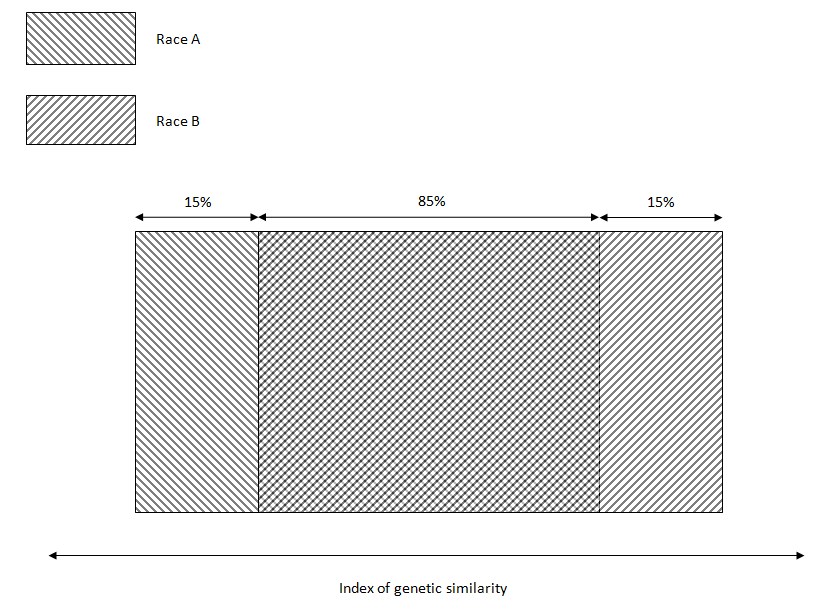
which is complete nonsense. And that is the point! To the unenlightened, Lewontin’s sound bite means that Race A people are often more similar genetically to Race B people than to their co-ethnics. This mistaken intuition allows Lewontin to claim, “Since such racial classification is now seen to be of virtually no genetic or taxonomic significance either, no justification can be offered for its continuance”.

Lewontin’s fallacy is this: he wasn’t looking for clusters in DNA-space. And identifying clusters of objects with correlated properties is the only way we can parse the world!

Some horses have brown hair, and so do some humans. Other humans have blond hair. So counting hair colour only, humans and horses overlap substantially. Yet as more dimensions of thingspace are counted—number of legs, intelligence, top speed and so on—horses and humans diverge into two highly distinct clusters.

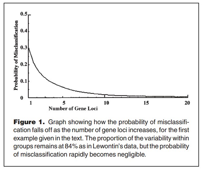
Different continental races are less clearly separate in DNA-space than humans and horses are in DNA-space or broader thingspace, but the same idea applies. Counting only one gene, there’s a lot of overlap on average; there aren’t many monoracial alleles. But as more gene loci are counted, the weight of cumulative similarity begins to separate the races.

“Lewontin’s Fallacy” was coined by one A.W.F. Edwards in 2003. Here is his illustration:

The mere ability to classify people into races using their genes is unremarkable. Nigerians and Swedes can be discriminated almost perfectly using skin colour, so even the handful of genes coding for skin colour must be a sufficient tell-tale. It doesn’t follow that Swedes and Nigerians are necessarily distant in DNA-space, where all DNA bases are taken into account. But Lewontin’s 15% is an Fst statistic—(an estimate of) genetic distance between populations, averaged across all gene loci—so it doesn’t privilege genes coding for visible, racially distinctive features.

Edwards’s point is that 15% between-population variation, averaged across all gene loci, makes populations distant from one another (at least on average) in gene-space. Although not as comprehensive as DNA-space, gene-space is an unbiased proxy.

We can also make Lewontin’s “15%” more tangible. Henry Harpending proves in Kinship and Population Subdivision (2002) that Fst, the measure Lewtonin refers to, is approximately equal to “kinship”.

In genetics, the coefficient of kinship between two individuals is “the probability that an allele taken randomly from one will be identical to an allele taken at the same locus from another”. Typically, the coefficient of kinship between parent and child is 0.25; the kinship of grandparents and grandchildren is 0.125. An individual’s kinship with himself is only 0.5, because humans are diploid (we have two presumably unrelated sets of chromosomes).

Or to provide a better definition, kinship is similarity in excess of “background” allele-sharing within some population. Because a parent passes on genes to his children, they are similar in excess of the alleles random individuals have in common. A homogenous background population is the usual assumption.

It helps to imagine a “landscape of kinship”. The individual and any identical twins are a mountain peak; from the peak there’s an abrupt fall to the base camp of nuclear family, and a slighter smaller fall to the level of nephews, nieces, uncles and so on. Descending further, we soon hit the flat plain of an ethnic group (at least, it’s flat on our map). Travelling further from the mountain, we tread gently downhill. But there’s occasionally a steep decline or cliff in the kinship landscape, corresponding to some natural or cultural barrier to gene-flow. These steep gradients roughly demarcate racial and ethnic groups.

Kinship within a nuclear family is 0.25 if measured as elevation above the ideally flat plain of the family’s ethnic group. But their kinship is even higher than this when measured against more distant, lower ground in the kinship landscape. Also, plugging the Japanese-Mbuti Fst into Harpending’s equations (NB: Eq. 2 on p.146 contains a typo), the kinship of an Mbuti grandfather and his half-Japanese grandchild is less than his kinship with another random Mbuti (not that this need bear on their emotional relationship).

Lewontin’s “15%” signifies kinship of 0.15 between an individual and co-ethnics who aren’t close family, when compared to distant points in humanity’s kinship topography. On a German individual’s map, the elevation difference of ~0.15 between random Nigerians and Germans is even bigger than the elevation difference of 0.125 between his grandson and other Germans. Far from being negligible, 15% is a very large value.

For the icing on the cake, Lewtonin’s apportionment of diversity within and between populations can also be applied to families. Henry Harpending proves, in the appendix to a Frank Salter article (Salty does have his uses), that 75% of genetic variation is within nuclear families and only 25% is between nuclear families. I doubt many people consider the nuclear family a genetically insubstantial category.

III) Racial boundaries

Lewontin’s statistic fails to refute the concept of race, and actually proves that the magnitude of human genetic variation is large. Nonetheless, it remains to be shown that races—population-scale genetic clusters—actually exist.

Cavalli-Sforza’s Fst data testify that on average, humans of distant geographical ancestry are commensurately distant in DNA-space. But genetic variation might yet be perfectly continuous between these extremes. Consider the electromagnetic spectrum: gamma rays and radio waves obviously aren’t the same thing. However, the decrease in wavelength from radio waves to gamma rays is perfectly continuous; there are no gaps in the spectrum, creating naturally distinct categories of radiation. Likewise, human populations might be highly distinct without being clustered. Clustering implies a low-density region of thingspace separating high-density regions; although human genetic variation exists, it might just be spread across DNA-space in uniform density. Zimbabweans are distant from Norwegians in this spread, but there might not be “thin air” between them.

Another way of putting it: maybe variation is purely clinal. Fortunately, we have studies to tell us the answer. From Clines, Clusters and the Effect of Study Design on the Inference of Human Population Structure, Rosenberg et al (2005):

“Previously, we observed that without using prior information about individual sampling locations, a clustering algorithm applied to multilocus genotypes from worldwide human populations produced genetic clusters largely coincident with major geographic regions. It has been argued, however, that the degree of clustering is diminished by use of samples with greater uniformity in geographic distribution, and that the clusters we identified were a consequence of uneven sampling along genetic clines. Expanding our earlier dataset from 377 to 993 markers, we systematically examine the influence of several study design variables—sample size, number of loci, number of clusters, assumptions about correlations in allele frequencies across populations, and the geographic dispersion of the sample—on the “clusteredness” of individuals. With all other variables held constant, geographic dispersion is seen to have comparatively little effect on the degree of clustering. Examination of the relationship between genetic and geographic distance supports a view in which the clusters arise not as an artifact of the sampling scheme, but from small discontinuous jumps in genetic distance for most population pairs on opposite sides of geographic barriers, in comparison with genetic distance for pairs on the same side. Thus, analysis of the 993-locus dataset corroborates our earlier results: if enough markers are used with a sufficiently large worldwide sample, individuals can be partitioned into genetic clusters that match major geographic subdivisions of the globe, with some individuals from intermediate geographic locations having mixed membership in the clusters that correspond to neighboring regions.”

In other words, it’s what you’d expect from facial appearance—duh. Human genetic variation isn’t perfectly smooth; the Sahara creates an abrupt difference between Algerians and Nigerians, relative to the distance between these countries. This demarcates fuzzy “caucasoid” and “negroid” races. But Somalis have significant membership in both clusters. Both sides of the clusters vs. clines debate commit the fallacy of grey: old-fashioned views of race propose too-sharp clusters, and those race denialists who aren’t just smitten with Lewontin posit unrealistically smooth variation.

If all human DNA-codes are plotted in thingspace, there are high-density regions corresponding to families, and more diffuse high-density regions corresponding to various concentric circles of kinship. There are also regions within humanity’s volume of DNA-space where relatively few humans are dotted. The geographic barrier of the Himalayas, for example, begets a sparsely populated volume in DNA-space between the dense East and South Asian clusters.

It remains to be proved that these clusters align with traditional continental races. But they do; from Worldwide Human Relationships Inferred from Genome-Wide Patterns of Variation, Li at al (2008):

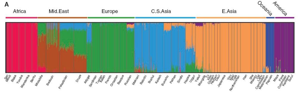
In other words, one tells the software how many clusters it should distinguish, and (if one chooses K=7) it tries to cleave human DNA-space into the 7 most natural clusters. It then assigns cluster membership to each individual; mixed membership may signify mixing of populations, or simply that clusters are fuzzy at the edges.

Despite taking no account of race, whatever the value of K these humanity-wide analyses identify traditional racial and ethnic divisions. Clustering analyses within continental races are less clean-cut. That’s because on a smaller geographic scale, genetic barriers like the English channel are insubstantial and any clusters are correspondingly vague. Variation still isn’t perfectly smooth, but the viewing lens of clinality becomes relatively useful in comparable to clustering.

One might object that the arbitrary choice of K renders structure analysis too subjective. It doesn’t really; consider the picture below (of course, thingspace and DNA-space have a lot more than two dimensions):

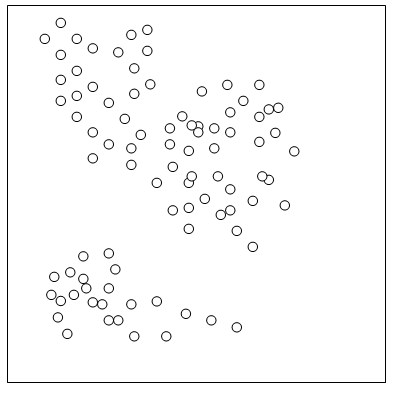
I’ve drawn two clusters of circles. Or are there three?

Analysis with K=2 would cleanly separate the bottom group from the top. With K=3, the top group would also split along its obvious join, although a few intermediate circles would have partial membership in both clusters. At K=4 and higher, any clustering is vague. To assign more than three components to the circles would make them look like the Mid. East individuals above: mixed up.

Attempts to cleave reality where there aren’t joints will make a mess; otherwise, to “arbitrarily” speak of either two or three clusters in this picture is no more arbitrary than to distinguish tits from sparrows, whilst also distinguishing blue tits from great tits. There isn’t a choice to be made, whether to distinguish two clusters or three; rather, there are both two andthree well-defined clusters.

If there weren’t 2, 3, 4 and 5 meaningful population clusters within humanity, the software simply wouldn’t produce orderly results when asked to cleave DNA-space at K = 2, 3, 4 and 5. The tidy-looking ancestry of most individuals in Li et al evinces a natural division of humanity into continental races, not a biased method.

IV) Variation within races

The existence of population-level clusters doesn’t imply that individuals are always most similar to their co-ethnics. There must be random variation, and proximity between borderline members of each cluster. In Genetic Similarities Within and Between Human Populations, Witherspoon et al (2007) attempt to resolve this question:

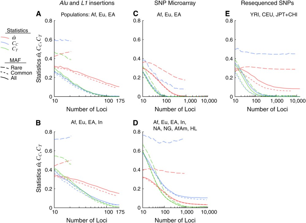
The statistic  is the dissimilarity fraction: an estimator of the probability that a pair of individuals randomly chosen from different populations are genetically more similar than an independent pair chosen from any single population. At  = 0, individuals are always more similar to members of their own population than to members of other populations; at the maximum  = 0.5, individuals are as likely to be more similar to members of other populations as to members of their own.

Cc is the centroid misclassification rate. Individuals are compared to the centroid of each population rather than to every other individual. The centroid is the genetic average of a population, an individual whose pseudogenotypes at each locus are the frequencies of the genotypes in that population. Cc is the proportion of individuals classified to the wrong population using this method. The expected value of Cc is 1 – 1/n, where n is the number of populations.

Ct is the population trait value misclassification rate. This is a measure designed to be highly effective in assigning individuals to populations, but a less natural measure of their overall genetic similarity.

The diagram shows Witherspoon et al’s results for these statistics using various populations and numbers of loci. Unsurprisingly, they found that rates of misclassification decrease as more loci are added. To quote:

“Thus the answer to the question “How often is a pair of individuals from one population genetically more dissimilar than two individuals chosen from two different populations?” depends on the number of polymorphisms used to define that dissimilarity and the populations being compared. The answer, can be read from Figure 2. Given 10 loci, three distinct populations, and the full spectrum of polymorphisms (Figure 2E), the answer is  ≅0.3, or nearly one-third of the time. With 100 loci, the answer is ∼20% of the time and even using 1000 loci, ≅10%. However, if genetic similarity is measured over many thousands of loci, the answer becomes “never” when individuals are sampled from geographically separated populations.

On the other hand, if the entire world population were analyzed, the inclusion of many closely related and admixed populations would increase This is illustrated by the fact that and the classification error rates, Cc and Ct, all remain greater than zero when such populations are analyzed, despite the use of >10,000 polymorphisms (Table 1, microarray data set; Figure 2D).”

Europeans, sub-Saharan Africans and East Asians are always more genetically similar to co-ethnics than to individuals from the other two populations. Overall, this paper buttresses race realism.

Witherspoon et al’s results do suggest a degree of overlap between less geographically distinct ethnic groups. Including African Americans, Africans and Hispano-Latinos as different “populations” in Figure 2D confounds things a little, but Figure 2E with the Chinese and Japanese also has a non-zero  despite 10,000 loci.

Then again, 10,000 loci isn’t the full dimensionality of DNA-space. Since misclassification tends to decrease as more loci are added, inter-ethnic proximity in a comprehensive DNA-space might be even rarer than Witherspoon et al found.

V) Humans are 99.9% genetically identical

Whether or not this statistic is strictly true, humans are very similar. But this is no basis for refuting race realism. If the maximum 0.1% difference is trivial, ethnic and familial genetic similarities are insignificant. Even identical twins are scarcely more similar than two random humans, if a 0.1% difference can be ignored.

For perspective, Chimpanzees share about 98% of our DNA; bananas share about 50%. Clustering in thingspace doesn’t require differences in all or even most dimensions—otherwise, humans and chimps would be inseparable.

VI) The purpose of racial classification

Why does all of this matter?

I know genes are inherently valuable to Salterians. But the rest of us are more concerned with their function. In particular, racial differences in intelligence and temperament are important, if they exist.

I believe that Oceanians, Native Americans and sub-Saharan Africans are substantially inferior to other humans in intelligence. I form this conclusion due to: lack of geniuses amongst people with high membership in these clusters; consistent failure to achieve and sustain civilisation; predictable sinking to the bottom of multi-ethnic societies; and my intelligence estimate of the representative negroes I’ve encountered. (Incidentally, I expect IQ does measure intelligence, but I don’t regard it as strong evidence. The methodology of global IQ testing is questionable, and the Flynn effect casts doubt on the whole business.)

If sub-Saharan Africans, Oceanians and Native Americans weren’t clusters in human gene-space or DNA-space, this belief would be weakened. We don’t know which genes code for intelligence. In the absence of population-level clusters, low intelligence might still be related to nominal sub-Saharan ancestry and negro physical traits, but this would be a coincidence. Why shouldn’t the distribution of low mean intelligence spread in a funny shape, covering sub-Saharan Africa only sporadically? If one can generalise from Nigerian to Nigerian scarcely more than from Nigerian to Swede, are our observations sufficient to make sweeping claims about sub-Saharan intelligence?

Yet if negro appearance and sub-Saharan ancestry imply membership of a cluster in DNA-space, racial generalisations gain credence.

Witherspoon et al say the following:

“To the extent that phenotypically important genetic variation resembles the variation studied here, we may extrapolate from genotypic to phenotypic patterns. Resequencing studies of gene-coding regions show patterns similar to those seen here (e.g., STEPHENS et al. 2001), and many common disease-associated alleles are not unusually differentiated across populations (LOHMUELLER et al. 2006). Thus it may be possible to infer something about an individual’s phenotype from knowledge of his or her ancestry.

However, consider a hypothetical phenotype of biomedical interest that is determined primarily by a dozen additive loci of equal effect whose worldwide distributions resemble those in the insertion data set (e.g., with  = 0.15; Table 1). Given these assumptions, the genetic distance used in computing  and Cc is equivalent to a phenotypic distance, so Figure 2 can be used to analyze this hypothetical trait. Figure 2A shows that a trait determined by 12 such loci will typically yield = 0.31 (0.20–0.41) and Cc= 0.14 (0.054–0.29; medians and 90% ranges). About one-third of the time ( = 0.31) an individual will be phenotypically more similar to someone from another population than to another member of the same population. Similarly, individuals will be more similar to the average or “typical” phenotype of another population than to the average phenotype in their own population with a probability of ∼14% (Cc= 0.14). It follows that variation in such a trait will often be discordant with population labels.”

The number of genes coding for intelligence is thought to be very large. From the abstract of Genome-wide association studies establish that human intelligence is highly heritable and polygenic, Davies et al (2011):

“Data from twin and family studies are consistent with a high heritability of intelligence, but this inference has been controversial. We conducted a genome-wide analysis of 3511 unrelated adults with data on 549 692 single nucleotide polymorphisms (SNPs) and detailed phenotypes on cognitive traits. We estimate that 40% of the variation in crystallized-type intelligence and 51% of the variation in fluid-type intelligence between individuals is accounted for by linkage disequilibrium between genotyped common SNP markers and unknown causal variants. These estimates provide lower bounds for the narrow-sense heritability of the traits. We partitioned genetic variation on individual chromosomes and found that, on average, longer chromosomes explain more variation. Finally, using just SNP data we predicted ~1% of the variance of crystallized and fluid cognitive phenotypes in an independent sample (P=0.009 and 0.028, respectively). Our results unequivocally confirm that a substantial proportion of individual differences in human intelligence is due to genetic variation, and are consistent with many genes of small effects underlying the additive genetic influences on intelligence.”

Because intelligence is determined by the small effects of many genes—substantially more than a dozen—the expected values of and Cc for this phenotype are particularly low. Continental races undoubtedly overlap in the final product of intelligence, but overlap in intelligence-coding–DNA-space is probably small. It therefore makes sense to generalise mean intelligence estimates across continental races.

If intelligence were determined by three or four genes, Gabonese people might easily be much smarter than other sub-Saharans. Maybe they lucked out and a couple of different, high-intelligence alleles are common in their local area. But since intelligence is determined by the small effects of maybe a hundred or more genes, the scope for variation decreases. Particularly in the absence of strong selection pressure and barriers to gene flow, overall frequencies of intelligence-coding alleles are likely to be similar in the tribes of Gabon, Cameroon and the Congo, creating similar intelligence distributions.

Strong countervailing evidence can refute such a generalisation. Pygmies are much smaller than surrounding populations, even though height is very polygenic (albeit forest-dwelling humans experience predictable selection pressure for small stature, and high barriers to gene flow). But until Gabonese, Namibian or Ugandan geniuses start cropping up the best bet is that, generalising our observations of sub-Saharans, they just aren’t very smart.